Show Shapes¶

Here we briefly show how to call the dataset functions in tadasets as well as a simple plotting utility.

[1]:

import tadasets
import matplotlib.pyplot as plt

[2]:

t = tadasets.torus(n=2000, c=10, a=2)
tadasets.plot3d(t)

[2]:

<Axes3D: >

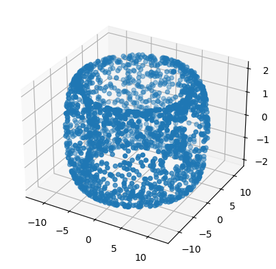
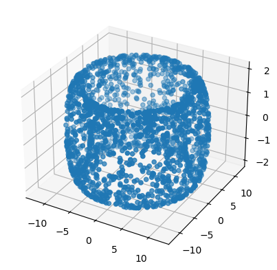
The torus now includes an option for more uniform sampling. This method uses rejection sampling to ensure that the number of points in a region is roughly proportional to the area of that region.

[3]:

t = tadasets.torus(n=2000, c=10, a=2, uniform=True)
tadasets.plot3d(t)

[3]:

<Axes3D: >

[3]:

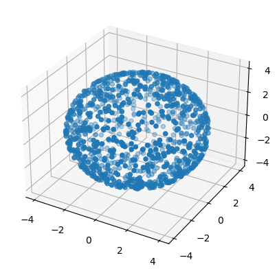
t = tadasets.sphere(n=1000, r=4)
tadasets.plot3d(t)

[3]:

<Axes3D: >

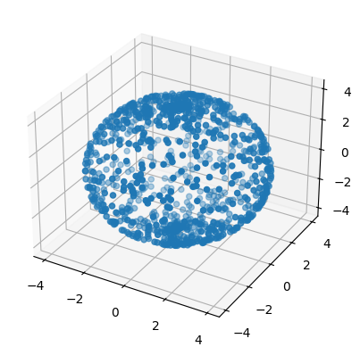
Similarly, sphere also has an option for more uniform sampling. This method simply uses independent guassians to uniformly sample the sphere.

[4]:

t = tadasets.sphere(n=1000, r=4, uniform=True)
tadasets.plot3d(t)

[4]:

<Axes3D: >

[4]:

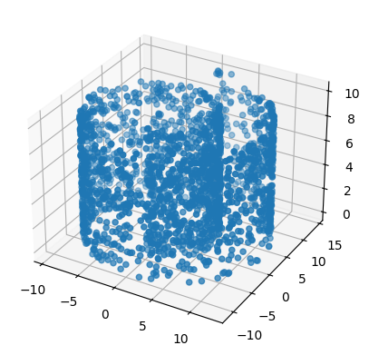
t = tadasets.swiss_roll(n=2000)
tadasets.plot3d(t)

[4]:

<Axes3D: >

[5]:

t = tadasets.infty_sign()
plt.scatter(t[:, 0], t[:, 1])
plt.show()

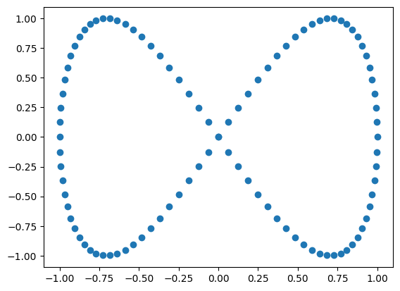
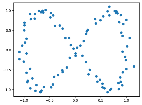
The noise parameter corresponds to the standard deviation of Gaussian noise applied to a dataset. For the above “infinity sign” dataset, we see the efect of noise=0.05 below.

[6]:

t = tadasets.infty_sign(noise=0.05)
plt.scatter(t[:, 0], t[:, 1])
plt.show()

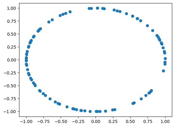
[7]:

t = tadasets.dsphere(d=1)
plt.scatter(t[:, 0], t[:, 1])
plt.show()

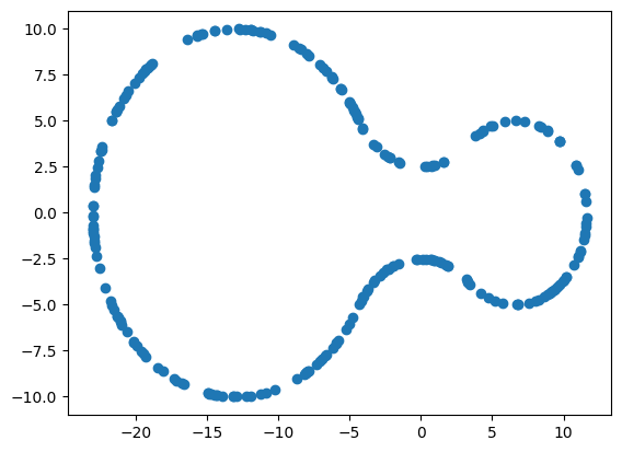
[8]:

t = tadasets.eyeglasses(n=250, r1=10, r2=5)
plt.scatter(t[:, 0], t[:, 1])
plt.show()